Grover's Algorithm
Summary
Grover’s algorithm is a search algorithm for unstructured databases. It is provably optimal for quantum computers, and quadratically faster than the best classical algorithm. Lov Grover published his algorithm in “A fast quantum mechanical algorithm for database search” (1996)
This page sets up unstructured search as a problem to be solved by Grover’s Algorithm, describes the algorithm’s basic operating principles, and takes the reader through a full example that uses the algorithm to solve NP-Complete problems.
Contents
- Preamble
- Grover's Algorithm
- Using Grover's Algorithm
- Computational Search
- Example: SAT Problems
- SAT Problems
- Building an Oracle
- More about Quantum Search
- Search for Unknown Number of Solutions
- Something Else?
- Exploiting Structure
- Combining with Classical Algorithms
- Nested Quantum Search
Preamble
Unstructured Search
A phonebook is an example of a structured database; Since a phonebook is sorted alphabetically, if given a name, we can quickly (in logarithmic time) locate that person’s phone number. Even if the phonebook has a large number of entries we can still find the name we’re looking pretty quickly. We will cover structured search in it’s own dedicated section.
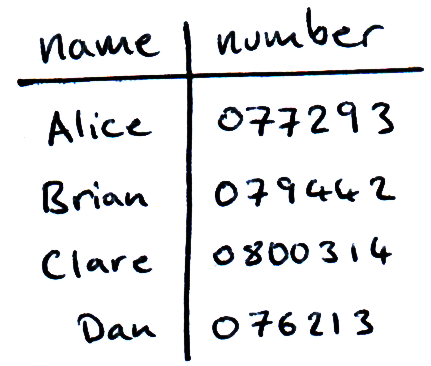
But if we turn the problem around, i.e. we are given a phone number and asked to find it’s corresponding name, the search problem suddenly becomes very difficult. We can make no educated guesses about where the number we’re looking for might be. The best classical algorithm for unstructured search is ‘random guessing’, where we pick out entries at random until we happen upon the phone number we’re looking for. This algorithm grows linearly with the number of entries (N) in the phonebook, since it will take (on average) N/2 queries of the database to find the correct entry.
Thinking about Unstructured Search like a Computer
Since there is absolutely no way to search a real phonebook using Grover’s algorithm, we need to think about database search like a computer scientist. Firstly, to help ease the transition to quantum circuits, we will assume the names and numbers in our phonebook are stored in binary, and we will call them ‘inputs’ and ‘outputs’ respectively. Now note that the number of entries we have in our database (N) is related to the number of bits (n) by N = 2n.
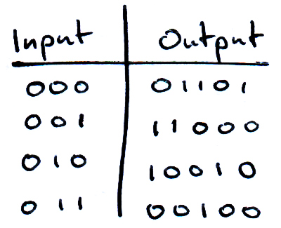
By convention, we call the output we’re looking for ‘ω’.
The Query Circuit
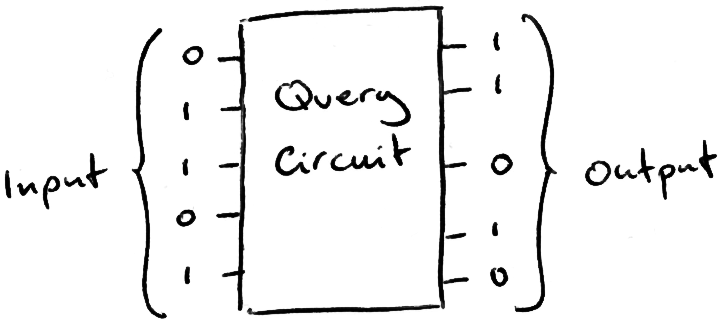
The query circuit is a function that takes an address (the name) as input, and outputs the data at that address (the phone number). At the moment we treat the query circuit as a ‘black box’, which means we do not care about how it works, but we will do later.
To perform a random guessing search, we input random addresses into the query circuit and check the output, repeating with different binary strings until the output equals the data we’re looking for. We add a ‘checker’ circuit that flips a ‘flag’ bit if our output is ω.
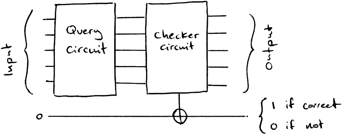
Using our phonebook analogy, we put random names into the query circuit until it outputs the phone number we were given. This algorithm has a complexity of order 2n (exponential time).
Grover's Algorithm
Outline
Here we will quickly describe Grover’s algorithm in a high-level way.
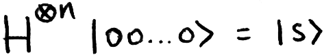
The first step of the algorithm is to initialise the starting state |s⟩, a superposition of all possible inputs. We know this can be easily accomplished using a Hadamard transform on each qubit.
Since we want our algorithm to output ω, we want our qubits to be as close to the state |ω⟩ as possible when we measure them. The algorithm is tasked with moving the state of the qubits from |s⟩ to |ω⟩. To simplify, we can split every state in our computation into one of two categories: |ω⟩ and not |ω⟩. Since we only care about |ω⟩ and all the states that are not |ω⟩, we can plot this on a 2D graph:
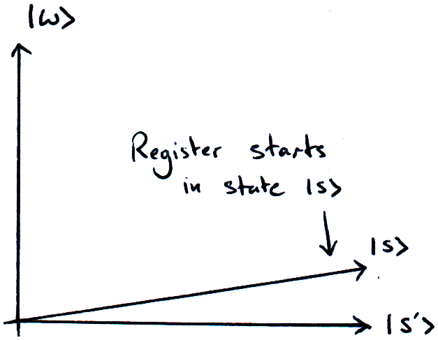
Where |s’⟩ is the equal superposition of all states excluding |ω⟩. This means |s’⟩ is perpendicular to |ω⟩. Our computer is never actually in the state |s’⟩ (if it is then we’re doing something very wrong!), we just use |s’⟩ to act as the axis on our graph, and to illustrate the reflections we are doing.
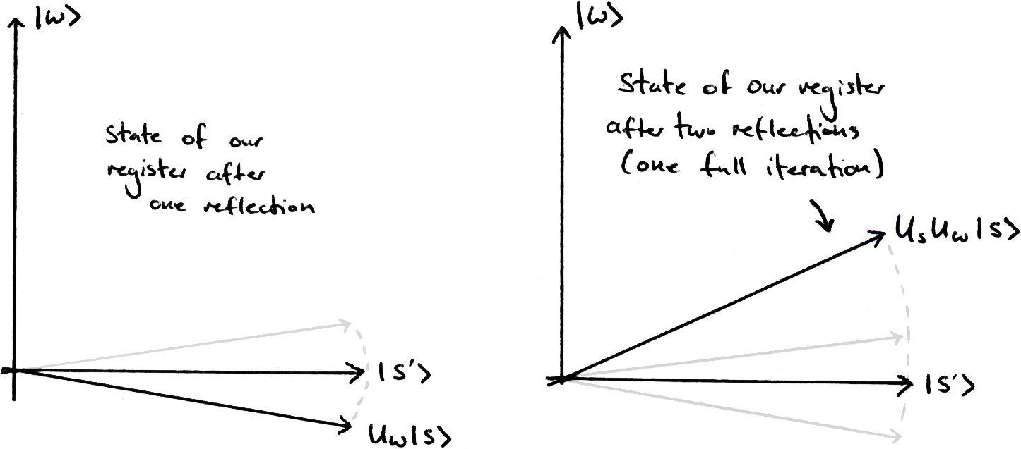
We perform a reflection around |s’⟩ (this operator is called ‘Uω’) and a reflection around |s⟩ (called ‘Us’), and repeat until we are close to |ω⟩. This takes ~2n/2 repetitions.
Implementing Grover's Algorithm as a Quantum Circuit
Here we will go through each step and show how they can be performed by a universal quantum computer. The first step, initialising the state |s⟩ is very simple: We do a Hadamard transform (H-gate) on each qubit, this gives us a uniform superposition of every state.
The Quantum Oracle
(A very cool title)
The second operation, the reflection around |s’⟩ is the most interesting step, this is where our query circuit comes in. To perform the reflection, we need a circuit that adds a negative phase to the |ω⟩ component of our vector.
Firstly, we implement our classical query circuit as a quantum circuit, (how we actually do this depends on the problem and we will cover this later,) this means we can pass it our superposition of inputs to get a new equal superposition of output states.
And use our checker circuit to add a negative phase to the state we’re searching for. In the image below, our |ω⟩ is the state |1010⟩. This is easy enough to check for, we just use a Toffoli gate with the appropriate controls.
But how do we apply the negative phase? Remember that if we apply an X-gate to a qubit in the |-⟩ state, we get back a qubit in the state -|-⟩:
So we use our checker circuit to apply an X-gate to a |-⟩ qubit. We then reverse the classical query circuit to get back our initial |s⟩, except the |ω⟩ component is negative.
We describe the combined state of the search qubits and the |-⟩ qubit using the Kronecker product (link to section). This explains how the negative phase introduced with the checker circuit applies to the whole state:
And remember that any states that are not |ω⟩ will not activate the checker circuit and will pass through unaffected. This whole circuit is a functioning oracle, it performs a reflection about |s’⟩ as specified in Grover’s algorithm.
The Diffusion Operator
The next step is the reflection through |s⟩, this step is actually really simple, and is the same for every database search. This reflection is called the ‘Diffusion Operator’. To perform the diffusion operator we need to invert anything perpendicular to |s⟩, and we do this following a similar method to the Oracle.
We will do the transformation that turns |s⟩ into the all-zeroes vector |000..0⟩, and invert anything that is not |000..0⟩, before transforming back again. Before, we easily created |s⟩ by applying a H-gate to each qubit, if we want to go back the all-zeroes vector we just apply a H-gate to each qubit again.
The whole diffusion operator looks like this:
Note that we have applied a negative phase to all the states that are parallel to |s⟩, not perpendicular as we specified. Since global phase can be ignored (link to global phase), this is completely equivalent. We now have all the steps required to complete Grover’s algorithm.
As a full Quantum Circuit
We can combine our classical query circuit, checker circuit and diffusion operator to complete the first iteration of Grover’s algorithm:
Simple! We then repeat this O(√N) times.
Example Circuit in Quirk
Here is an example circuit in Quirk
The bottom 4 qubits are the work qubits, which output the answer. The qubit above the work qubits is the |-⟩ qubit we use to add the negative phase, and the top qubit is used for labels.
Our algorithm searches for |0101⟩. Watch how the probability of measuring |0101⟩ grows with each iteration, and reaches 90.8% chance after two iterations. Classically (with random guessing) we would have a ~13% chance of getting |0101⟩ after two guesses.